Develop a simulation of response of the slider-crank mechanism shown in the picture over a period of 2 seconds. The data for the problem is as follows:
Crank length = 0.2m, crank mass = 1kg.
Connecting rod length = 0.5m, connecting rod mass = 3kg.
Slider mass = 2kg.
Spring constant = 10000 N/m, unstretched length = 0.5m.
Viscous damping coefficient = 1000 Ns/m

Connecting rod length = 0.5m, connecting rod mass = 3kg.
Slider mass = 2kg.
Spring constant = 10000 N/m, unstretched length = 0.5m.
Viscous damping coefficient = 1000 Ns/m

Case 2:
The crank is being driven at a constant angular speed of 60 rpm clockwise.
The starting crank angle is 30 degrees above the horizontal
Constaint Equations:
As derived in Case 1

In case 2, we need to find all initial values for the
velocities by differentiating the constraint equation,

The last equation is added to case 2 because of the applied
constant initial angular velocity to the crank.


The following m-file is used to find the initial values of
velocities and accelerations of all of the three bodies.
clear all;

L1=0.2;
L2=0.5;
g=9.81;
w=-2*pi

q= zeros(9,1);              % Initial Positions

q(3)=pi/6;
q(6) =-asin(0.2);
q(1)=L1/2*cos(q(3));
q(2) =L1/2*sin(q(3));
q(4) =L1*cos(q(3))+L2/2*cos(q(6));
q(5) =L1*sin(q(3))+L2/2*sin(q(6));
q(7) =L1*cos(q(3))+L2*cos(q(6));
q(8) =0;
q(9) =0

qdotc  =zeros(9,9); % The coefficient matrix of initial velocities

qdotc(1,1)=1;
qdotc(1,3)=q(2);%L1/2*sin(q(3));
qdotc(2,2)=1;
qdotc(2,3)=-q(1); %L1/2*cos(q(3));
qdotc(3,4)=1;
qdotc(3,3)=2*q(2);%L1*sin(q(3));
qdotc(3,6)=L2/2*sin(q(6));
qdotc(4,5)=1;
qdotc(4,3)=-2*q(1); %L1*cos(q(3));
qdotc(4,6)=-L2/2*cos(q(6));
qdotc(5,7)=1;
qdotc(5,3)=2*q(2); %L1*sin(q(3));
qdotc(5,6)=L2*sin(q(6));
qdotc(6,8)=1;
qdotc(6,3)=-2*q(1); %L1*cos(q(3));
qdotc(6,6)=-L2*cos(q(6));
qdotc(7,8)=1;
qdotc(8,9) =1;
qdotc(9,3)=1;

qdotR=zeros(9,1); % Right side of initial velocity matrix
qdotR(9)=w;

B = inv(qdotc);

qdot = inv(qdotc)*qdotR % Initial Velocities for the given w

 qddc           = zeros(9,9); % Coeffecient matrix of acceleration
    qddc(1,1) =1;
    qddc(1,3) =L1/2*sin(q(3));
    qddc(2,2) =1;
    qddc(2,3) = -L1/2*cos(q(3));
    qddc(3,3) =L1*sin(q(3));
    qddc(3,4)=1;
    qddc(3,6) =L2/2*sin(q(6));
    qddc(4,3) =-L1*cos(q(3));
    qddc(4,5) =1;
    qddc(4,6) =-L2/2*cos(q(6));
    qddc(5,3) =L1*sin(q(3));
    qddc(5,6) =L2*sin(q(6));
    qddc(5,7) =1;
    qddc(6,3) =-L1*cos(q(3));
    qddc(6,6) =-L2*cos(q(6));
    qddc(6,8) =1;
    qddc(7,8) =1;
    qddc(8,9)=1;
    qddc(9,3)=1;

    qddR =zeros(9,1); % Right side of acceleration matrix
    qddR(1) =-qdot(3)^2*L1/2*cos(q(3));
    qddR(2) =-qdot(3)^2*L1/2*sin(q(3));
    qddR(3) = -qdot(3)^2*L1*cos(q(3))-qdot(6)^2*L2/2*cos(q(6));
    qddR(4) =-qdot(3)^2*L1*sin(q(3))-qdot(6)^2*L2/2*sin(q(6));
    qddR(5) =-qdot(3)^2*L1*cos(q(3))-qdot(6)^2*L2*cos(q(6));
    qddR(6) =-qdot(3)^2*L1*sin(q(3))-qdot(6)^2*L2*sin(q(6));

    E=inv(qddc);

    qdd =E*qddR  % Intial accelerations
The result of this file is:

Now we need to simulate the position and velocities of the
three bodies using constraint equation and differentiating them.


MATLAB Codes for Case 2:
function zdot = Project_2(t,z)
% Function to evaluate the derivatives for the SliderCrank Mechanism
% Separate position and velocity information
q = z( 1: 9); % position data
qdot = z( 10: 18); % velocity data
% Acceleration of gravity
g = 9.81; % Units - m/sec.^2
% Input torgue
tau = 0; % Units - N m
%Spring and Damper Constants
k = 10000; % Spring constant Units N/m
c = 1000; % Dashpot constant Units - Ns/m
% Rigid Body Data
m1 = 1; % Units - Kg
m2 = 3; % Units - Kg
m3 = 2; % Units - Kg
L1 = 0.2; % Units - m
L2 = 0.5; % Units - m
I1 = (1/12)*m1*L1^2; % Units - Kg m^2
I2 = (1/12) * m2 * L2^2; % Units - Kg m^2
I3 = 0; % Units - Kg m^2
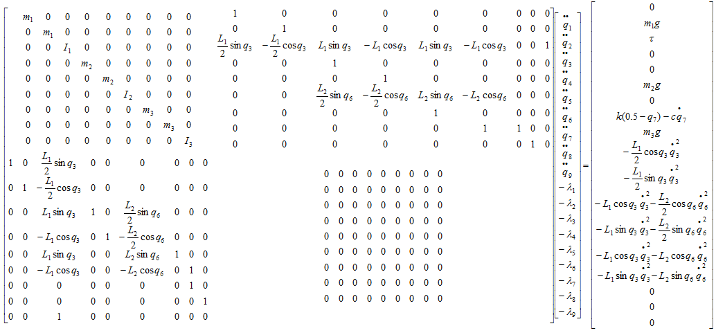
% Build the Mass matrix
M = zeros( 9, 9);
M( 1, 1) = m1;
M( 2, 2) = m1;
M( 3, 3) = I1;
M( 4, 4) = m2;
M( 5, 5) = m2;
M( 6, 6) = I2;
M( 7, 7) = m3;
M( 8, 8) = m3;
M( 9, 9) = I3;
% Specify the generalized forces
Q = zeros( 9,1);
Q( 2) = -m1*g;
Q( 3) = tau;
Q( 5) = -m2*g;
Q( 7) = k*(0.5-q(7))-c*qdot(7);
Q( 8) = -m3*g;
% Specify the derivative of the constraint matrix
Phiq = zeros( 9,9);
% Body 1
Phiq( 1, 1) = 1;
Phiq( 1, 3) = L1/2*sin(q(3));
Phiq( 2, 2) = 1;
Phiq( 2, 3) = -L1/2*cos(q(3));
Phiq( 3, 3) = L1*sin(q(3));
Phiq( 3, 4) = 1;
Phiq( 3, 6) = L2/2*sin(q(6));
%**********************************************************************
% Body 2
Phiq( 4, 3) = -L1*cos(q(3));
Phiq( 4, 5) = 1;
Phiq( 4, 6) = -L2/2*cos(q(6));
Phiq( 5, 3) = L1*sin(q(3));
Phiq( 5, 6) = L2*sin(q(6));
Phiq( 5, 7) = 1;
Phiq( 6, 3) = -L1*cos(q(3));
Phiq( 6, 6) = -L2*cos(q(6));
Phiq( 6, 8) = 1;
%**********************************************************************
%Body 3
Phiq( 7, 8) = 1;
Phiq( 8, 9) = 1;
Phiq(9,3) =1;
%**********************************************************************
% Right Side of Constraint Equation
Phiqdot = zeros( 9,1);
Phiqdot( 1) = (L1/2)*cos(q(3))*qdot(3)^2;
Phiqdot( 2) = (L1/2)*sin(q(3))*qdot(3)^2;
Phiqdot( 3) = L1*cos(q(3))*qdot(3)^2+L2/2*cos(q(6))*qdot(6)^2;
Phiqdot( 4) = L1*sin(q(3))*qdot(3)^2+L2/2*sin(q(6))*qdot(6)^2;
Phiqdot( 5) = L1*cos(q(3))*qdot(3)^2+L2*cos(q(6))*qdot(6)^2;
Phiqdot( 6) = L1*sin(q(3))*qdot(3)^2+L2*sin(q(6))*qdot(6)^2;
% Build Coefficient Matrix
C = [M Phiq';Phiq zeros( 9,9)];
D = inv(C);
% Build Right Vector
R = [ Q' -Phiqdot']';
% FInd Solution
ACC = D*R;;
qdd = ACC(1: 9);
% Determine the time derivative of the state zector
zdot = [qdot' qdd']';
close all;
clear all;
% Class Example
% Set the parameters
Tspan = 0.0:0.0001:2;
g = 9.81;
L1 = 0.2;
L2 = 0.5;
theta1 = pi/6;
theta2 = 2.940235-pi;
% Determine the initial conditions
q = zeros(9,1);
q(1) = 0.2/2*cos(theta1);
q(2) = 0.2/2*sin(theta1);
q(3) = theta1;
q( 4) = 2*(.1*cos(theta1))+0.5/2*cos(theta2);
q( 5) = -0.5/2*sin(theta2);
q(6) = theta2;
q(7) = 2*(0.1*cos(theta1))+0.5*cos(theta2);
qdot = zeros(9,1); % All initial velocities are zero
qdot(1) = 0.3142;
qdot(2)=-0.5441;
qdot(3)=-2*pi;
qdot(4)=0.7394;
qdot(5)=-0.5441;
qdot(6)=2.2214;
qdot(7)=0.8505;
Z0 = [q' qdot']'; % Initial Condition Vector
options = odeset('RelTol',1.0e-9,'AbsTol',1.0e-6);
[Tout,Z] = ode45(@Project_2,Tspan,Z0,options);
% Body 1
x1 = Z(:,1);
y1 = Z(:,2);
Theta1 = Z(:,3);
figure(1);
plot(Tout, x1, 'k', Tout, y1,'k--');
grid on;
title('Crank Position');
xlabel('Time - seconds');
ylabel('Position - meters');
legend('Horizontal Position','Vertical Position');
figure(2);
plot(Tout, Theta1, 'k');
grid;
title('Angle of Crank');
xlabel('Time - seconds');
ylabel('Angle - radians');
x1dot = Z(:,1+ 9);
y1dot = Z(:,2+ 9);
Theta1dot = Z(:,3+ 9);
figure(3);
plot(Tout, x1dot, 'k', Tout, y1dot, 'k--', Tout, Theta1dot,'k-.');
grid;
title('Velocities of Crank');
xlabel('Time - seconds');
ylabel('Velocities - meters/s and angular velocity - rad/sec.');
legend('Horizontal Velocity','Vertical Velocity', 'Angular Velocity');
% Connecting Rod
x2 = Z(:,4);
y2 = Z(:,5);
Theta2 = Z(:,6);
figure(4);
plot(Tout, x2, 'k', Tout, y2,'k--',Tout,Theta2,'k-.');
grid;
title('Connecting Rod Position');
xlabel('Time - seconds');
ylabel('Position - meters and angle - rad');
legend('Horizontal Position','Vertical Position','Angular Position');
x2dot = Z(:,4+ 9);
y2dot = Z(:,5+ 9);
Theta2dot = Z(:,6+ 9);
figure(5);
plot(Tout, x2dot, 'k', Tout, y2dot, 'k--', Tout, Theta2dot,'k-.');
grid;
title('Velocities of Connection Rod');
xlabel('Time - seconds');
ylabel('Velocities - meters/s and angular velocity - rad/sec.');
legend('Horizontal Velocity','Vertical Velocity', 'Angular Velocity');
% Slider
x3 = Z(:,7);
y3 = Z(:,8);
Theta3 = Z(:,9);
figure(6);
plot(Tout, x3, 'k', Tout, y3,'k--',Tout,Theta3,'k-.');
grid;
title('Slider Position');
xlabel('Time - seconds');
ylabel('Position - meters and angle - rad');
legend('Horizontal Position','Vertical Position','Angular Position');
x3dot = Z(:,7+ 9);
y3dot = Z(:,8+ 9);
Theta3dot = Z(:,9+ 9);
figure(7);
plot(Tout, x3dot, 'k', Tout, y3dot, 'k--', Tout, Theta3dot,'k-.');
grid;
title('Velocities of Slider');
xlabel('Time - seconds');
ylabel('Velocities - meters/s and angular velocity - rad/sec.');
legend('Horizontal Velocity','Vertical Velocity', 'Angular Velocity');
Results of Case 2


Your can find the solution for Case 1 by clicking here...

